Data visualization/데이터시각화(R)
데이터시각화(R)_Diamonds
뉴욕킴
2023. 9. 20. 23:16
geom_text 를 이용하여 그림 안에 글자를 넣기
library(tidyverse)df=data.frame(trt=c("a","b","c"),resp=c(1.2,3.4,2.5))df
ggplot(df,aes(trt,resp))+geom_point()
- 점대신 a,b,c로 잡아주기
ggplot(df,aes(trt,resp))+geom_text(aes(label=trt))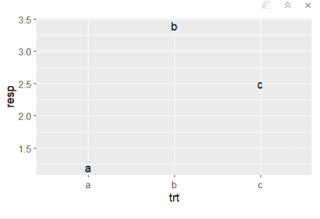
- 기존의 글씨체인 "고딕체"로 나오는 것 확인
ggplot(df,aes(resp,trt))+geom_text(aes(label=trt))
- 폰트 바꾸기(family 이용)
- family: 문자의 폰트를 지정. (“sans”(기본값,고딕체), “serif”(바탕체), “mono”
ggplot(df,aes(resp,trt))+geom_text(aes(label=trt),family="mono")
- fontface:서체를 지정. (“plain”(기본값), “bold”, “italic”)
ggplot(df,aes(resp,trt))+geom_text(aes(label=trt),fontface="bold")
- 이태리체로 변경
ggplot(df,aes(resp,trt))+geom_text(aes(label=trt),fontface="italic",family="serif")
점 찍는 위치 표시 방법
- 산점도 그리기
ggplot(df,aes(resp,trt))+geom_point()
ggplot(df,aes(resp,trt))+geom_text(aes(label=trt))
- 텍스트와 점 같이 찍기
ggplot(df,aes(resp,trt))+geom_point()+geom_text(aes(label=trt))
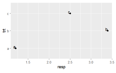
- hjust (“left”, “center”(기본값), “right”, “inward”, “outward”) 와 vjust (“bottom”, “middle”(기본값), “top”, “inward”, “outward”) aesthetics 을 이용하여 문자의 정렬 형태를 조정
- 가로의 위치 지정
ggplot(df,aes(resp,trt))+geom_point()+geom_text(aes(label=trt),hjust="right")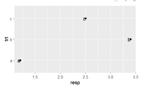
- 왼쪽으로 위치 지정
ggplot(df,aes(resp,trt))+geom_point()+geom_text(aes(label=trt),hjust="left")
- 위에 찍기
ggplot(df,aes(resp,trt))+geom_point()+geom_text(aes(label=trt),hjust="left", vjust='top')
df <- data.frame(trt = c("a", "b", "c"), resp = c(1.2, 3.4, 2.5))
ggplot(df, aes(resp, trt)) +
 geom_point()+
 geom_text(aes(label = trt),hjust="right",vjust="bottom")
- “inward”를 이용하면 모두 그림영역안에 표시된다
df <- data.frame(x = c(1, 2, 1, 2, 1.5),
 y = c(1, 1, 2, 2, 1.5),
 text = c( "bottom-left","bottom-right","top-left","top-right","center"),
 S=c(6,8,10,12,14),
 a=c(0,30,45,60,90))
ggplot(df, aes(x, y)) + geom_text(aes(label = text))
ggplot(df, aes(x, y)) +
 geom_text(aes(label = text), vjust = "inward", hjust = "inward")
- size: 글씨의 크기
ggplot(df, aes(x,y)) +
 geom_point() +
 geom_text(aes(label = text),size=7)
- angle: 문자의 회전
ggplot(df, aes(x,y)) +
 geom_point() +
 geom_text(aes(label = text),size=7,angle=30)
ggplot(df, aes(x,y)) + geom_point() +
 geom_text(aes(label = text, angle=a),size=7)
ggplot(df, aes(x,y)) + geom_point() +
 geom_text(aes(label = text, angle=a,size=S))
- x와 y limit 바꾸기 (범위 바꾸기)
ggplot(df, aes(x,y)) + geom_point() +
 geom_text(aes(label = text, angle=a,size=S))+xlim(0,3)
ggplot(df, aes(x,y)) + geom_point() +
 geom_text(aes(label = text, angle=a,size=S))+xlim(0,3)+ylim(0,3)
- check_overlap = TRUE 를 이용하면 겹쳐지는 label 을 제거해 준다. 단, 자료의 순서대로 label 을 쓰면서 겹치는 부분을 제거하므로 뒤쪽 자료의 label 이 제거됨
ggplot(mpg, aes(displ, hwy)) +
 geom_text(aes(label = model)) +
 xlim(1, 8)
ggplot(mpg, aes(displ, hwy)) +
 geom_text(aes(label = model), check_overlap = TRUE) +
 xlim(1, 8)
- directlables 패키지의 geom_dl() 함수를 이용하면 범주의 이름을 적절한 위치에 써준다.
ggplot(mpg, aes(displ, hwy, colour = class)) +
 geom_point()
ggplot(mpg, aes(displ, hwy, colour = class)) +
 geom_point(show.legend = FALSE) +
 directlabels::geom_dl(aes(label = class), method = "smart.grid")
선/영역/문자 등을 이용하여 그림에 주석달기
- geom_line(): 자료를 x 변수의 순서대로 sorting 후 점을 이어줌
- geom_path(): 자료에 나타난 순서대로 점을 이어줌
df <- data.frame(
 x = c(6, 2, 12),
 y = c(4, 8, 12),
 label = c("a","b","c")
)
p = ggplot(df, aes(x, y, label = label)) +
labs(x = NULL, y = NULL)p+geom_line()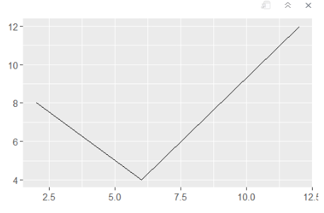
p+geom_line()+geom_text()
p+geom_line()+geom_text()+ggtitle("line")
- geom_area(): geom_line 으로 그려진 선과 y=0 으로 만들어지는 영역을 나타냄
- geom_polygon(): 자료에 나타난 순서대로 점을 잇고 마지막 점과 첫 점을 이어 생기는 영역을 나타냄
- geom_rect(): x 와 y 축의 범위로 지정된 네점(xmin, xmax, ymin, ymax)를 이어주는 영역을 나타냄
p+geom_rect(aes(xmin=5,xmax=6,ymin=6,ymax=10))
p+geom_area()
p+geom_polygon()
- geom_vline(): 지정된 위치(xintercept)에 수평선을 그려줌
- geom_hline(): 지정된 위치(yintercept)에 수직선을 그려줌
- geom_abline(): 지정된 intercept 와 slope 를 이용하여 직선을 그려줌
p+geom_point(size=5,color="green")+
 geom_vline(xintercept=5,size=2)+
 geom_hline(yintercept=10,linetype=2)+
 geom_abline(intercept=0,slope=1,size=1.5,linetype=2,color="red")
- economics 자료를 이용하여 실업자수의 변동 추이를 집권당에 따라 달라지는지를 알아보기 위한 그림 그리기
ggplot(economics,aes(date,unemploy))+geom_line()
Example data: presidential data (’ggplot2` library)
– 1953 년부터 2017 년까지의 미국 대통령 임기와 집권당을 나타낸 자료
– 변수들 - name : 대통령 이름 - start : 임기 시작일 - end : 임기 종료일 - party : 집권 정당
range(economics$date)[1] "1967-07-01" "2015-04-01"- 자료 준비
presidential1 = subset(presidential, start > economics$date[1])

presidential1
- 시각화 진행
ggplot(economics)+geom_line(aes(date,unemploy))
ggplot(economics) +
 geom_rect(
 aes(xmin = start, xmax = end, fill = party),
 ymin = -Inf, ymax = Inf, alpha = 0.2,
 data = presidential1
 ) +
 geom_vline(
 aes(xintercept = as.numeric(start)),
 data = presidential1,
 colour = "grey50", alpha = 0.5
 ) +
 geom_text(
 aes(x = start, y = 2500, label = name),
 data = presidential1,
 size = 3)
gplot(economics) +
 geom_rect(
 aes(xmin = start, xmax = end, fill = party),
 ymin = -Inf, ymax = Inf, alpha = 0.2,
 data = presidential1
 ) +
 geom_vline(
 aes(xintercept = as.numeric(start)),
 data = presidential1,
 colour = "grey50", alpha = 0.5
 ) +
 geom_text(
 aes(x = start, y = 2500, label = name),
 data = presidential1,
 size = 3, vjust = 0, hjust = 0, nudge_x = 50
 ) +
 geom_line(aes(date, unemploy)) +
 scale_fill_manual(values = c("blue", "red"))
- annotate()을 이용하여 그림 안에 주석 달기
yrng <- range(economics$unemploy)
xrng <- range(economics$date)
caption <- paste(strwrap("Unemployment rates in the US have
 varied a lot over the years", 40), collapse = "\n")
ggplot(economics) +
 geom_rect(
 aes(xmin = start, xmax = end, fill = party),
 ymin = -Inf, ymax = Inf, alpha = 0.2,
 data = presidential1
 ) +
 geom_vline(
 aes(xintercept = as.numeric(start)),
 data = presidential1,
 colour = "grey50", alpha = 0.5
 ) +
 geom_text(
 aes(x = start, y = 2500, label = name),
 data = presidential1,
 size = 3, vjust = 0, hjust = 0, nudge_x = 50
 ) +
 geom_line(aes(date, unemploy)) +
 scale_fill_manual(values = c("blue", "red")) +
 annotate("text", x = xrng[1], y = yrng[2], label = caption,
 hjust = "left", vjust = "top", size = 4)
- geom_abline()을 이용한 보조선 넣기
diamonds
ggplot(diamonds,aes(carat,price))+geom_point()
ggplot(diamonds, aes(log10(carat), log10(price))) +
 geom_bin2d() +
 facet_wrap(~cut, nrow = 1)
mod_coef <- coef(lm(log10(price) ~ log10(carat), data = diamonds))
ggplot(diamonds, aes(log10(carat), log10(price))) +
 geom_bin2d() +
 geom_abline(intercept = mod_coef[1], slope = mod_coef[2],
 colour = "white", size = 1) +
 facet_wrap(~cut, nrow = 1)