데이터시각화(R)_Tips
library(reshape2)library(tidyverse)data(tips)head(tips) total_bill tip sex smoker day time size
1 16.99 1.01 Female No Sun Dinner 2
2 10.34 1.66 Male No Sun Dinner 3
3 21.01 3.50 Male No Sun Dinner 3
4 23.68 3.31 Male No Sun Dinner 2
5 24.59 3.61 Female No Sun Dinner 4
6 25.29 4.71 Male No Sun Dinner 4summary(tips) total_bill tip sex smoker
Min. : 3.07 Min. : 1.000 Female: 87 No :151
1st Qu.:13.35 1st Qu.: 2.000 Male :157 Yes: 93
Median :17.80 Median : 2.900
Mean :19.79 Mean : 2.998
3rd Qu.:24.13 3rd Qu.: 3.562
Max. :50.81 Max. :10.000
day time size
Fri :19 Dinner:176 Min. :1.00
Sat :87 Lunch : 68 1st Qu.:2.00
Sun :76 Median :2.00
Thur:62 Mean :2.57
3rd Qu.:3.00
Max. :6.00
Q. 성별에 따라 tip의 지불 성향이 차이가 있을까?
- 연속형인지 범주형인지 확인하기: violin, boxplot 사용
ggplot(tips,aes(sex,tip))+geom_violin()+geom_boxplot()
ggplot(tips,aes(sex,tip))+geom_violin()+geom_boxplot(width=0.1)# width=0.1 → boxplot 크기

→ 후한 팁을 주는 건 남자다. 하지만 피크는 남자가 낮다
- geom_jitter(): geom_point()에서 각각의 점의 위치를 범위 내에서 무작위로 수평분산 시켜
ggplot(tips,aes(sex,tip))+geom_violin()+geom_boxplot(width=0.1)+geom_jitter(color='grey70')
- t.test : 두 집단 간의 평균값이 유의미하게 다른지 여부를 검정
- 귀무가설 H0: 두 그룹의 평균값이 같다.
- 대립가설 H1: 두 그룹의 평균값이 다르다.
t.test(tip~sex,data=tips)Welch Two Sample t-test
data: tip by sex
t = -1.4895, df = 215.71, p-value = 0.1378
alternative hypothesis: true difference in means between group Female and group Male is not equal to 0
95 percent confidence interval:
-0.5951448 0.0828057
sample estimates:
mean in group Female mean in group Male
2.833448 3.089618 - t값: t-test 통계량(t 값 음수: 첫 번째 그룹의 평균값이 더 적다/ t 값 양수: 첫 번째 그룹의 평균값이 더 크다)
- df: 자유도(degree of freedom)
- p-value: 유의확률
→ p-value 값이 0.05보다 작으면, 귀무가설을 기각하고 대립가설을 채택함.
(p-value 값이 0.05보다 크면 귀무가설을 기각하지 않고, 두 그룹 간의 평균값이 유의미하게 다르지 않다는 것 확인
- tiprate 라는 새로운 변수 만들기
- tiprate: tip열을 total_bill로 나눈 값(각 식사 대금에 대한 팁의 비율 계산)
tips$tiprate = tips$tip/tips$total_billhead(tips)ggplot(tips,aes(sex,tiprate))+geom_violin()+geom_boxplot(width=0.1)+geom_jitter(color='grey70')
→ tip이 후한 건 여자들이다.
t.test(tiprate~sex,data=tips) Welch Two Sample t-test
data: tiprate by sex
t = 1.1433, df = 206.76, p-value = 0.2542
alternative hypothesis: true difference in means between group Female and group Male is not equal to 0
95 percent confidence interval:
-0.006404119 0.024084498
sample estimates:
mean in group Female mean in group Male
0.1664907 0.1576505
Q. smoker 여부에 따라 지불 성향이 차이가 있을까?
sex열의 두 범주 (예: 남성과 여성) 사이에서
tiprate의 평균에 유의미한 차이가 있는지를 확인하기 위한 것입니다. 검정 결과는 t-통계량(t-statistic), 자유도(degrees of freedom), p-값(p-value) 등을 포함하는 가설검정 결과를 출력할 것입니다. p-값이 유의수준보다 작으면, 평균의 차이가 통계적으로 유의미하다는 것을 나타냅니다.
- t.test
- tiprate~sex: tiprate를 sex에 따라 그룹화 한다.
- data=tips: 데이터셋으로 tips 데이터프레임을 사용한다.
- var.equal=TRUE: 두 그룹의 분산이 같다고 가정한다.
t.test(tiprate~sex,data=tips,var.equal=TRUE)Two Sample t-test
data: tiprate by sex
t = 1.0834, df = 242, p-value = 0.2797
alternative hypothesis: true difference in means between group Female and group Male is not equal to 0
95 percent confidence interval:
-0.007232898 0.024913277
sample estimates:
mean in group Female mean in group Male
0.1664907 0.1576505
ggplot(tips,aes(smoker,tiprate))+geom_violin()+geom_boxplot(width=0.1)+geom_jitter(color='grey70')
→ Yes는 자유로운 영혼들로 보임
Q. 요일에 따라 tip 지불 성향이 차이가 있을까?
t.test(tiprate~smoker,data=tips,var.equal=TRUE)Two Sample t-test
data: tiprate by smoker
t = -0.47967, df = 242, p-value = 0.6319
alternative hypothesis: true difference in means between group No and group Yes is not equal to 0
95 percent confidence interval:
-0.01975024 0.01201507
sample estimates:
mean in group No mean in group Yes
0.1593285 0.1631960 ggplot(tips,aes(day,tiprate))+geom_violin()+geom_boxplot(width=0.1)+geom_jitter(color='grey70')
→ 목요일: 비즈니스 미팅이 많아 평균 15%에 있는 것으로 추정
→ 금요일: 샘플 사이즈가 작음
→ 토/일: 주말은 가족들과 외식이 잦아 테이블이 지저분해서 팁을 많이 주는 것으로 추정
- lm : 선형회귀분석 수행하는 코드
lm(formula = tiprate ~ day, data = tips)- formula = tiprate ~ day: 이 부분은 모델의 수식 또는 공식을 정의합니다. 여기서 종속 변수인 tiprate와 독립 변수인 day 사이의 관계를 나타내는 모델을 만듭니다. 이것은 "tiprate를 day에 대한 함수로 예측하라"는 의미입니다.
- data = tips: 이 부분은 데이터를 제공하는 데이터프레임을 지정합니다. 여기서는 tips 데이터프레임을 사용하여 모델을 만듭니다.
- tapply() : 주어진 데이터를 그룹화하고 각 그룹 내에서 평균을 계산
tapply(tips$tiprate,tips$day,mean) Fri Sat Sun Thur
0.1699130 0.1531517 0.1668973 0.1612756
- 이 명령은 tapply() 함수를 사용하여 주어진 데이터를 그룹화하고 각 그룹 내에서 평균을 계산합니다. 구체적으로는 tips 데이터프레임에서 tiprate를 day 별로 그룹화하고, 각 그룹 내에서 평균을 계산합니다. 이것은 day에 따른 tiprate의 평균을 출력합니다.
Q. 성별, smoker 여부에 따라 지불 성향이 차이가 있을까?
ggplot(tips,aes(smoker,tiprate))+geom_violin()+geom_boxplot(width=0.1)+geom_jitter(color="grey70")+facet_wrap(~sex)
- anova: 분산 분석을 수행하는데 사용
anova(lm(tiprate~smoker, data = tips))Analysis of Variance Table
Response: tiprate
Df Sum Sq Mean Sq F value Pr(>F)
smoker 1 0.00086 0.0008609 0.2301 0.6319
Residuals 242 0.90548 0.0037417 anova(lm(tiprate~smoker+sex, data = tips))Analysis of Variance Table
Response: tiprate
Df Sum Sq Mean Sq F value Pr(>F)
smoker 1 0.00086 0.0008609 0.2302 0.6318
sex 1 0.00439 0.0043857 1.1730 0.2799
Residuals 241 0.90110 0.0037390 anova(lm(tiprate~smoker*sex, data = tips))Analysis of Variance Table
Response: tiprate
Df Sum Sq Mean Sq F value Pr(>F)
smoker 1 0.00086 0.0008609 0.2330 0.62972
sex 1 0.00439 0.0043857 1.1872 0.27699
smoker:sex 1 0.01448 0.0144780 3.9191 0.04888 *
Residuals 240 0.88662 0.0036943
---
Signif. codes:
0 ‘***’ 0.001 ‘**’ 0.01 ‘*’ 0.05 ‘.’ 0.1 ‘ ’ 1- lm(tiprate ~ smoker * sex, data = tips): 이 부분은 tips 데이터 프레임을 기반으로 한 선형 회귀 모델을 만듭니다. 종속 변수는 tiprate이며, 독립 변수로는 smoker와 sex를 사용하고 이들 간의 상호작용도 포함합니다. 따라서 이 모델은 tiprate를 smoker와 sex의 조합으로 예측하려고 합니다.
- anova(): 이 함수는 분산 분석(ANOVA)을 수행합니다. 여기서는 위에서 생성한 선형 회귀 모델을 분석하고자 합니다.
따라서 이 코드는 tiprate를 smoker와 sex의 조합에 따라 예측하는 선형 회귀 모델에 대한 분산 분석을 수행하고, 이러한 독립 변수들 간의 상호작용이 tiprate에 미치는 영향을 평가하려고 합니다. ANOVA 결과를 통해 변수들 간의 통계적 유의성을 확인할 수 있습니다.
Q. total_bill과 tip과의 관계(전체 자료에서)
ggplot(tips,aes(total_bill,trip)+geom_point()
       +geom_smooth(method = "lm")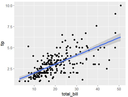
- total_bill에 대한 평균이기 때문에 중앙값을 이어주면 생각보다 낮게 나옴
- 선 아래: 평균보다 낮게 줌, 선 위: 평균보다 많이 줌
- 단순선형회귀 모델을 사용하여 tip과 total_bill 사이의 관계를 분석
summary(lm(tip~total_bill,data=tips))Call:
lm(formula = tip ~ total_bill, data = tips)
Residuals:
    Min      1Q  Median      3Q     Max
-3.1982 -0.5652 -0.0974  0.4863  3.7434
Coefficients:
Estimate Std. Error t value Pr(>|t|)
(Intercept) 0.920270 0.159735 5.761 2.53e-08 ***
total_bill 0.105025 0.007365 14.260 < 2e-16 ***
---
Signif. codes:
0 ‘***’ 0.001 ‘**’ 0.01 ‘*’ 0.05 ‘.’ 0.1 ‘ ’ 1
Residual standard error: 1.022 on 242 degrees of freedom
Multiple R-squared: 0.4566, Adjusted R-squared: 0.4544
F-statistic: 203.4 on 1 and 242 DF, p-value: < 2.2e-16- Residuals(잔차: 예측된 값-실제값) → 회귀 모델의 적합도를 평가하는데 사용
Residuals:
Min 1Q Median 3Q Max
-3.1982 -0.5652 -0.0974 0.4863 3.7434 * 1사분위수, 중앙값, 제3사분위수, 최대값 순서
- Coefficients(회귀계수)
Coefficients:
            Estimate Std.Error t value Pr(>|t|)
(Intercept)   0.92027   0.159735   5.761   <2e-08 ***
total_bill    0.10503   0.007365 14.260    <2e-16 ***
* intercept : 절편 → tip이 total_bill이 없을 때의 추정치로서 약 0보다 크게 나타난다.
* total_bill 변수의 추정치
* Std.error : 표준 오차
* Signif.codes : p-value에 따라 유의미성(significance level)을 표시
- '***' : p-value < .001
- '**' : p-value < .01
- '*' : p-value < .05
- '.' : p-value < .1
- ' ' : p-value >= .1
- anova() 함수 분산분석 테이블 생성
- anova : 회귀 모델의 설명력과 변수들 간의 유의미한 차이를 평가하는데 사용
anova(lm(tip~total_bill,data=tips))Analysis of Variance Table
Response: tip
Df Sum Sq Mean Sq F value Pr(>F)
total_bill 1 212.42 212.424 203.36 < 2.2e-16 ***
Residuals 242 252.79 1.045
---
Signif. codes:
0 ‘***’ 0.001 ‘**’ 0.01 ‘*’ 0.05 ‘.’ 0.1 ‘ ’ 1- Df : total_bill에 대한 자유도 1
- Sum Sq : 제곱합이 약 212.42
- Mean Sq : 평균 제곱은 약 212.424
- F value : 약 203.36
- Residuals(잔차)에 대한 변수로, 자유도(Df)가 242, 제곱합(Sum Sq)은 약 252.79, 평균제곱(Mean Sq)는 약 1.045이다.
→ p < .001. F-value 값인 약 203.36은 모델의 설명력을 나타내며, 이 값이 크면 종속 변수의 tip을 예측하는데 독립변수인 total_bill이 유의미하게 기여한다는 것을 의미한다.
- cor: 상관계수 계산
cor(tips$total_bill,tips$tip)[1] 0.6757341- cor() 함수를 사용하여 tip과 total_bill간의 상관계수를 계산
- 계산된 상관계수 : 0.6757341
- summarize() : total_bill과 tip 사이의 상관계수를 요약
summarize(tips,cor=cor(total_bill,tip)) cor
1 0.6757341- tips와 total_bill 사이의 상관계수 값: 0.6757341
→ 팁과 총 지불액 간에 양의 선형적인 관계가 있음/ 상관계수 값이 0.5보다 크므로 관련성이 강한 정도라고 판단 가능
Q. total_bill과 tip 과의 상관관계(성별)
tips %>%
 ggplot(aes(total_bill,tip))+
 geom_point()+
 geom_smooth(method="lm")+facet_wrap(~sex)
summary(lm(tip~total_bill+sex+total_bill*sex,data = tips))Call:
lm(formula = tip ~ total_bill + sex + total_bill * sex, data = tips)
Residuals:
Min 1Q Median 3Q Max
-3.2232 -0.5660 -0.0977 0.4796 3.6675
Coefficients:
Estimate Std. Error t value Pr(>|t|)
(Intercept) 1.048020 0.272498 3.846 0.000154
total_bill 0.098878 0.013808 7.161 9.75e-12
sexMale -0.195872 0.338954 -0.578 0.563892
total_bill:sexMale 0.008983 0.016417 0.547 0.584778
(Intercept) ***
total_bill ***
sexMale
total_bill:sexMale
---
Signif. codes:
0 ‘***’ 0.001 ‘**’ 0.01 ‘*’ 0.05 ‘.’ 0.1 ‘ ’ 1
Residual standard error: 1.026 on 240 degrees of freedom
Multiple R-squared: 0.4574, Adjusted R-squared: 0.4506
F-statistic: 67.43 on 3 and 240 DF, p-value: < 2.2e-16
- 절편(intercept): 팁(tip)이 총 지불액(total_bill)과 성별에 따라서 약간 양의 상관관계가 있음을 나타내며 유의미한 것으로 나타납니다 (p < .001).
- total_bill: 총 지불액에 대한 회귀 계수로서 유의미하게 양의 상관관계가 있음을 나타내며 유의미한 것으로 나타납니다 (p < .001).
- sexMale: 성별에 대한 회귀 계수로서 유의미하지 않은 것으로 보입니다 (p > .05).
- total_bill:sexMale: 상호작용 항인 '총 지불액'과 '성별' 사이의 효과를 반영합니다만, 유의미하지 않은 것으로 보입니다 (p > .05).
→ 팁(tip)와 총 지불액(total_bill), 성별(sex) 사이에서 총체적인 설명력(Multiple R-squared = ~45%) 및 수정된 설명력(Adjusted R-squared = ~45%)이 확인되며,
종속 변수인 팁 (tip)를 예측하기 위해 독립 변수 중 하나인 '총 지불액' (total bill) 이 가장 크게 기여한다고 할 수 있습니다 (Pr(>|t|)).
anova(lm(tip~total_bill+sex+total_bill*sex,data = tips))Analysis of Variance Table
Response: tip
Df Sum Sq Mean Sq F value Pr(>F)
total_bill 1 212.424 212.424 201.9597 <2e-16 ***
sex 1 0.039 0.039 0.0369 0.8478
total_bill:sex 1 0.315 0.315 0.2994 0.5848
Residuals 240 252.435 1.052
---
Signif. codes:
0 ‘***’ 0.001 ‘**’ 0.01 ‘*’ 0.05 ‘.’ 0.1 ‘ ’ 1- total_bill : 자유도(Df), 제곱합(Sum Sq) 212.424, 평균제곱(Mean Sq) 212.424, F value 201.9597
→ 해석 결과로서 다중선형회귀 분석에서 총 지불액(total_bill) 변수는 팁(tip)과 유의미하게 관련되어 있음을 나타내며(p < .001), 성별(sex) 및 상호작용 항(total_bill:sexMale)`와 팁 사이에서는 유의미하지 않은 관련성을 나타냅니다 (p > .05)
Q. total_bill과 tip과의 관계(smoker로 나눴을 때)
ggplot(tips,aes(total_bill,tip))+
 geom_point()+
 geom_smooth(method="lm")+facet_wrap(~smoker)
- lm() : 다중선형회귀 모델
summary(lm(tip~total_bill+smoker+total_bill*smoker,data = tips))Call:
lm(formula = tip ~ total_bill + smoker + total_bill * smoker,
data = tips)
Residuals:
Min 1Q Median 3Q Max
-2.6789 -0.5238 -0.1205 0.4749 4.8999
Coefficients:
Estimate Std. Error t value Pr(>|t|)
(Intercept) 0.360069 0.202058 1.782 0.076012
total_bill 0.137156 0.009678 14.172 < 2e-16
smokerYes 1.204203 0.312263 3.856 0.000148
total_bill:smokerYes -0.067566 0.014189 -4.762 3.32e-06
(Intercept) .
total_bill ***
smokerYes ***
total_bill:smokerYes ***
---
Signif. codes:
0 ‘***’ 0.001 ‘**’ 0.01 ‘*’ 0.05 ‘.’ 0.1 ‘ ’ 1
Residual standard error: 0.9785 on 240 degrees of freedom
Multiple R-squared: 0.506, Adjusted R-squared: 0.4998
F-statistic: 81.95 on 3 and 240 DF, p-value: < 2.2e-16회귀 계수(coefficient) 부분에서 절편(intercept), total_bill, smokerYes, 그리고 total_bill:smokerYes(상호작용 항)에 대한 추정치(estimates), 표준 오차(std.error), t-value(t value), p-value(Pr(>|t|)) 등이 나타납니다.
- 절편(intercept): 팁(tip)이 총 지불액(total_bill)과 흡연 여부에 따라서 약간 양의 상관관계가 있음을 나타내며 유의미한 것으로 나타납니다 (p < .05).
- total_bill: 총 지불액에 대한 회귀 계수로서 유의미하게 양의 상관관계가 있음을 나타내며 유의미한 것으로 나타납니다 (p < .001).
- smokerYes: 흡연 여부에 대한 회귀 계수로서 팁과 유의미하게 관련되어 있음을 나타내며(p < .001),
- total_bill:smokerYes: 상호작용 항인 '총 지불액'과 '흡연 여부' 사이의 효과를 반영합니다(p < .001).
Signif.codes 부분은 p-value에 따라 유의미성(significance level)을 표시합니다.
'***' : p-value < .001
'**' : p-value < .01
'*' : p-value < .05
'.' : p-value < .1 -' ' : p-value >=
추가적인 정보로 잔차 표준오차(residual standard error), 결정계수(Multiple R-squared), 수정된 결정계수(Adjusted R-squared), F 통계량(F-statistic), 자유도(Degrees of Freedom), 그리고 F 통계량에 대한 p-value 등이 제공됩니다.
→ 해석 결과로서 다중선형회귀 분석 결과를 요약하면 다음과 같습니다:
팁(tip)와 총 지불액(total bill), 그리고 성별 (sex) 사이에서 전체적인 설명력(Multiple R-squared = ~50%) 및 수정된 설명력(Adjusted R-squared = ~50%) 이 확인되며,
종속 변수인 팁 (tip) 를 예측하기 위해 독립 변수 중 하나인 '총 지불 액' (`Total Bill') 이 가장 크게 기여한다고 할 수 있습니다 (Pr (>| t |)).
ANOVA 분석 결과 역시 전체적으로 유의미함을 보여주지만, 성별 ('sex') 및 상호 작용 항(total bill * sex)' 에서는 유의하지 않다고 할 수 있습니다(p > ..05)
Q. total_bill과 tip과의 관계(성별, smoker로 나눴을 때)
ggplot(tips,aes(total_bill,tip,group=1))+
 geom_point()+
 geom_smooth(method="lm")+facet_grid(sex~smoker)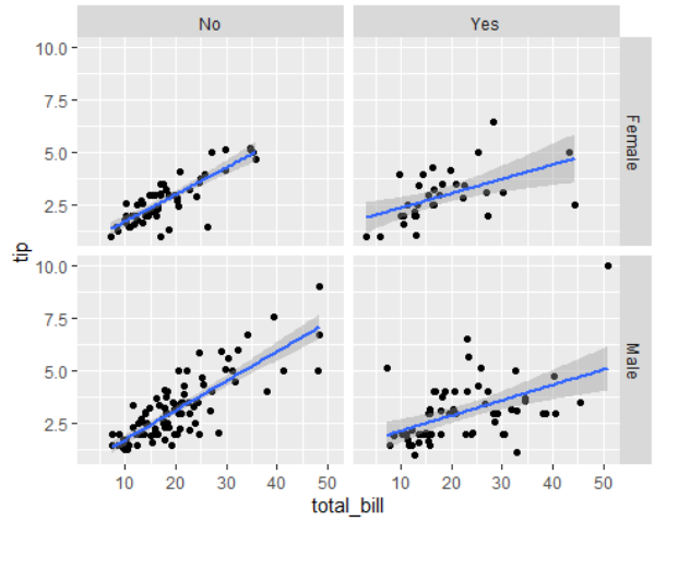
- 선을 기준으로 위: 팁을 후하게 줌
- 선을 기준으로 아래: 팁을 조금만 줌
summary(lm(tip~total_bill*smoker*sex,data = tips))lm(formula = tip ~ total_bill * smoker * sex, data = tips)
Residuals:
Min 1Q Median 3Q Max
-2.6506 -0.5288 -0.1095 0.4495 4.8676
Coefficients:
Estimate Std. Error t value
(Intercept) 0.451719 0.361449 1.250
total_bill 0.128239 0.018544 6.915
smokerYes 1.248849 0.525070 2.378
sexMale -0.103525 0.438711 -0.236
total_bill:smokerYes -0.059769 0.026494 -2.256
total_bill:sexMale 0.011479 0.021823 0.526
smokerYes:sexMale -0.171764 0.660720 -0.260
total_bill:smokerYes:sexMale -0.006989 0.031643 -0.221
Pr(>|t|)
(Intercept) 0.2126
total_bill 4.34e-11 ***
smokerYes 0.0182 *
sexMale 0.8137
total_bill:smokerYes 0.0250 *
total_bill:sexMale 0.5994
smokerYes:sexMale 0.7951
total_bill:smokerYes:sexMale 0.8254
---
Signif. codes:
0 ‘***’ 0.001 ‘**’ 0.01 ‘*’ 0.05 ‘.’ 0.1 ‘ ’ 1
Residual standard error: 0.9837 on 236 degrees of freedom
Multiple R-squared: 0.5091, Adjusted R-squared: 0.4945
F-statistic: 34.97 on 7 and 236 DF, p-value: < 2.2e-16
lm(tip~total_bill*smoker,data = tips)Call:
lm(formula = tip ~ total_bill * smoker, data = tips)
Coefficients:
(Intercept) total_bill
0.36007 0.13716
smokerYes total_bill:smokerYes
1.20420 -0.06757 - yes 그룹에서 intercept에 비해 total_bill은 작아짐을 확인
- total 1센트가 올라가면 tip은 6센트만 올라감
anova(lm(tip~total_bill*smoker*sex,data = tips))Analysis of Variance Table
Response: tip
Df Sum Sq Mean Sq F value
total_bill 1 212.424 212.424 219.5220
smoker 1 1.267 1.267 1.3094
sex 1 0.043 0.043 0.0447
total_bill:smoker 1 21.669 21.669 22.3932
total_bill:sex 1 0.211 0.211 0.2185
smoker:sex 1 1.182 1.182 1.2212
total_bill:smoker:sex 1 0.047 0.047 0.0488
Residuals 236 228.369 0.968
Pr(>F)
total_bill < 2.2e-16 ***
smoker 0.2537
sex 0.8328
total_bill:smoker 3.829e-06 ***
total_bill:sex 0.6406
smoker:sex 0.2702
total_bill:smoker:sex 0.8254
Residuals
---
Signif. codes:
0 ‘***’ 0.001 ‘**’ 0.01 ‘*’ 0.05 ‘.’ 0.1 ‘ ’ 1summary(lm(tip~total_bill,data = tips))Call:
lm(formula = tip ~ total_bill, data = tips)
Residuals:
Min 1Q Median 3Q Max
-3.1982 -0.5652 -0.0974 0.4863 3.7434
Coefficients:
Estimate Std. Error t value Pr(>|t|)
(Intercept) 0.920270 0.159735 5.761 2.53e-08 ***
total_bill 0.105025 0.007365 14.260 < 2e-16 ***
---
Signif. codes:
0 ‘***’ 0.001 ‘**’ 0.01 ‘*’ 0.05 ‘.’ 0.1 ‘ ’ 1
Residual standard error: 1.022 on 242 degrees of freedom
Multiple R-squared: 0.4566, Adjusted R-squared: 0.4544
F-statistic: 203.4 on 1 and 242 DF, p-value: < 2.2e-16
- 4개로 나눠서 보기
ggplot(tips,aes(total_bill,tip))+
  geom_point()+
  geom_smooth(method="lm")+facet_grid(sex~smoker)
lm(tip~total_bill,data = tips)
A=lm(tip~total_bill,data = tips)
coef(A)
tipsLmodel=coef(lm(tip~total_bill,data = tips))
tipsLmodel = coef(lm(tip~total_bill,data = tips))
ggplot(tips,aes(total_bill,tip,group=1))+
geom_point()+
geom_smooth(method="lm")+facet_grid(sex~smoker)+
geom_abline(intercept=tipsLmodel[1],slope=tipsLmodel[2],
linewidth = 1.5, color="red",alpha=0.5)