[3장-1] 분류 성능 평가 지표

Machine Learning/캐글스터디(파이썬 머신러닝)

[3장-1] 분류 성능 평가 지표

뉴욕킴 2023. 4. 4. 23:13

성능 평가 지표(Evaluation Metric)는 모델이 회귀인지 분류인지에 따라 여러 종류로 나뉨
1) 회귀의 경우 대부분 실제값과 예측값의 오차 평균값에 기반
2) 분류의 성능 평가 지표

분류 성능 평가지표: classification

- 정확도

- 오차행렬

- 정밀도

- 재현율

- F1 스코어

- ROC AUC

1) 정확도

정확도 : 실제 데이터에서 예측 데이터가 얼마나 같은지 판단하는 지표
= 예측 결과가 동일한 데이터 건수 / 전체 예측 데이터 건수
정확도는 직관적으로 모델 예측 성능을 나타내는 평가 지표이지만
이진 분류의 경우 정확도만으로 성능 평가하면 안됨 (ML 모델의 성능을 왜곡할 수 있기 때문)

import sklearn
print(sklearn.__version__) #버전 확인

1.0.2

import numpy as np
from sklearn.base import BaseEstimator # BaseEstimator 클래스를 상속받아 아무런 학습x

class MyDummyClassifier(BaseEstimator):
    # fit( ) 메소드는 아무것도 학습하지 않음.
    def fit(self, X , y=None):
        pass

    # predict( ) 메소드는 단순히 Sex feature가 1 이면 0 , 그렇지 않으면 1 로 예측함.
    def predict(self, X):
        pred = np.zeros( ( X.shape[0], 1 ))
        for i in range (X.shape[0]) :
            if X['Sex'].iloc[i] == 1:
                pred[i] = 0
            else :
                pred[i] = 1

        return pred

import pandas as pd
from sklearn.preprocessing import LabelEncoder

# Null 처리 함수
def fillna(df):
    df['Age'].fillna(df['Age'].mean(),inplace=True)
    df['Cabin'].fillna('N',inplace=True)
    df['Embarked'].fillna('N',inplace=True)
    df['Fare'].fillna(0,inplace=True)
    return df

# 머신러닝 알고리즘에 불필요한 피처 제거
def drop_features(df):
    df.drop(['PassengerId','Name','Ticket'],axis=1,inplace=True)
    return df

# 레이블 인코딩 수행.
def format_features(df):
    df['Cabin'] = df['Cabin'].str[:1]
    features = ['Cabin','Sex','Embarked']
    for feature in features:
        le = LabelEncoder()
        le = le.fit(df[feature])
        df[feature] = le.transform(df[feature])
    return df

# 앞에서 설정한 Data Preprocessing 함수 호출
def transform_features(df):
    df = fillna(df)
    df = drop_features(df)
    df = format_features(df)
    return df

import pandas as pd
from sklearn.model_selection import train_test_split
from sklearn.metrics import accuracy_score

# 원본 데이터를 재로딩, 데이터 가공, 학습데이터/테스트 데이터 분할.
titanic_df = pd.read_csv('./titanic_train.csv')
y_titanic_df = titanic_df['Survived']
X_titanic_df= titanic_df.drop('Survived', axis=1)
X_titanic_df = transform_features(X_titanic_df)
X_train, X_test, y_train, y_test=train_test_split(X_titanic_df, y_titanic_df, \
test_size=0.2, random_state=0)

# 위에서 생성한 Dummy Classifier를 이용하여 학습/예측/평가 수행.
myclf = MyDummyClassifier()
myclf.fit(X_train ,y_train)

mypredictions = myclf.predict(X_test)
print('Dummy Classifier의 정확도는: {0:.4f}'.format(accuracy_score(y_test , mypredictions)))

Dummy Classifier의 정확도는: 0.7877

→ 정확도는 불균형한(imbalanced) 레이블 값 분포에서 ML 모델의 성능을 판단할 경우, 적합한 평가 지표 X
예를 들어 100개의 데이터(90개는 0, 10개는 1)를 무조건 0으로 예측 결과를 반환하는 모델의 경우 정확도가 90% 임

평가의 지표로 정확도 사용 시 발생할 수 있는 문제점 (MNIST 데이터셋 활용)

* MNIST 데이터셋

- 0부터 9까지의 숫자 이미지의 픽셀 정보를 가지고 있음
- 이를 기반으로 숫자 Digit을 예측하는데 사용
- 사이킷런은 load_digits()를 API를 통해 MNIST 데이터셋 제공

from sklearn.datasets import load_digits
from sklearn.model_selection import train_test_split
from sklearn.base import BaseEstimator
from sklearn.metrics import accuracy_score
import numpy as np
import pandas as pd

class MyFakeClassifier(BaseEstimator):
    def fit(self,X,y):
        pass

    # 입력값으로 들어오는 X 데이터 셋의 크기만큼 모두 0값으로 만들어서 반환
    def predict(self,X):
        return np.zeros( (len(X), 1) , dtype=bool)

# 사이킷런의 내장 데이터 셋인 load_digits( )를 이용하여 MNIST 데이터 로딩
digits = load_digits()

print(digits.data)
print("### digits.data.shape:", digits.data.shape)
print(digits.target)
print("### digits.target.shape:", digits.target.shape)

[[ 0.  0.  5. ...  0.  0.  0.]
 [ 0.  0.  0. ... 10.  0.  0.]
 [ 0.  0.  0. ... 16.  9.  0.]
 ...
 [ 0.  0.  1. ...  6.  0.  0.]
 [ 0.  0.  2. ... 12.  0.  0.]
 [ 0.  0. 10. ... 12.  1.  0.]]
### digits.data.shape: (1797, 64)
[0 1 2 ... 8 9 8]
### digits.target.shape: (1797,)

digits.target == 7

array([False, False, False, ..., False, False, False])

# digits번호가 7번이면 True이고 이를 astype(int)로 1로 변환, 7번이 아니면 False이고 0으로 변환.
y = (digits.target == 7).astype(int)
X_train, X_test, y_train, y_test = train_test_split( digits.data, y, random_state=11)

# 불균형한 레이블 데이터 분포도 확인.
print('레이블 테스트 세트 크기 :', y_test.shape)
print('테스트 세트 레이블 0 과 1의 분포도')
print(pd.Series(y_test).value_counts())

# Dummy Classifier로 학습/예측/정확도 평가
fakeclf = MyFakeClassifier()
fakeclf.fit(X_train , y_train)
fakepred = fakeclf.predict(X_test)
print('모든 예측을 0으로 하여도 정확도는:{:.3f}'.format(accuracy_score(y_test , fakepred)))

레이블 테스트 세트 크기 : (450,)
테스트 세트 레이블 0 과 1의 분포도
0    405
1     45
dtype: int64
모든 예측을 0으로 하여도 정확도는:0.900

모든 예측을 0으로 하여도 정확도는 0.900

→ 이러한 문제를 해결하기 위해 오차행렬 사용

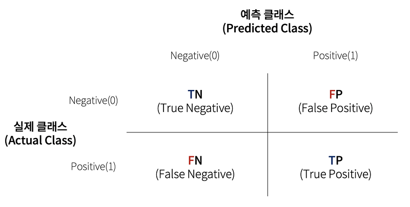
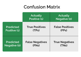
2. 오차행렬: confusion matrix

- 이진 분류의 예측 오류가 얼마인지와 함께 어떠한 유형의 예측 오류가 발생하고 있는지 함께 보여줌

-----------------------------------------------------------------

from sklearn.metrics import confusion_matrix

# 앞절의 예측 결과인 fakepred와 실제 결과인 y_test의 Confusion Matrix출력
confusion_matrix(y_test , fakepred)

array([[405,   0],
       [ 45,   0]], dtype=int64)

3. 정밀도와 재현율

정밀도와 재현율은 Positive 데이터셋의 예측 성능에 좀 더 초점을 맞춘 평가 지표

- 정밀도: TP / (FP+TP) / 예측을 Positive로 한 대상 중에 예측과 실제 값이 Positive로 일치한 비율

- 재현율: TP / (FN+TP) / 실제 값이 positive 인 대상 중에 예측과 실제 값이 Positive로 일치한 데이터의 비율

재현율이 중요한 경우
: 실제 Positive인 데이터 예측을 Negative로 잘못 판단하면 업무상 큰 영향있는 경우
정밀도가 중요한 경우
: 실제 Negative인 데이터 예측을 Positive로 잘못 판단하면 업무상 큰 영향있는 경우
가장 좋은 성능 평가는 재현율과 정밀도 모두 높은 수치를 얻는 것

# MyFakeClassifier의 예측 결과로 정밀도와 재현율 측정

from sklearn.metrics import accuracy_score, precision_score , recall_score

print("정밀도:", precision_score(y_test, fakepred))
print("재현율:", recall_score(y_test, fakepred))

정밀도: 0.0
재현율: 0.0

# 오차행렬, 정확도, 정밀도, 재현율을 한꺼번에 계산하는 함수 생성

from sklearn.metrics import accuracy_score, precision_score , recall_score , confusion_matrix

def get_clf_eval(y_test , pred):
    confusion = confusion_matrix( y_test, pred)
    accuracy = accuracy_score(y_test , pred)
    precision = precision_score(y_test , pred)
    recall = recall_score(y_test , pred)
    print('오차 행렬')
    print(confusion)
    print('정확도: {0:.4f}, 정밀도: {1:.4f}, 재현율: {2:.4f}'.format(accuracy , precision ,recall))

import numpy as np
import pandas as pd

from sklearn.model_selection import train_test_split
from sklearn.linear_model import LogisticRegression
import warnings
warnings.filterwarnings('ignore')

# 원본 데이터를 재로딩, 데이터 가공, 학습데이터/테스트 데이터 분할.
titanic_df = pd.read_csv('./titanic_train.csv')
y_titanic_df = titanic_df['Survived']
X_titanic_df= titanic_df.drop('Survived', axis=1)
X_titanic_df = transform_features(X_titanic_df)

X_train, X_test, y_train, y_test = train_test_split(X_titanic_df, y_titanic_df, \
test_size=0.20, random_state=11)

lr_clf = LogisticRegression(solver='liblinear')

lr_clf.fit(X_train , y_train)
pred = lr_clf.predict(X_test)
get_clf_eval(y_test , pred)

오차 행렬
[[108  10]
 [ 14  47]]
정확도: 0.8659, 정밀도: 0.8246, 재현율: 0.7705

4. Precision/ Recall Trade-off

정밀도와 재현율은 상호보완적인 평가지표로, 한쪽을 높이면 한쪽의 수치는 떨어지기 쉬움 : 트레이드오프
사이킷런의 분류 알고리즘은 예측 데이터가 특정 레이블(결정클래스값)에 속하는지를 계산하기 위해
먼저 개별 레이블별로 결정 확률을 구함 -> 예측 확률이 큰 레이블 값으로 예측하게 됨

# predict_proba( ) 메소드 확인, 2진 분류일때 0일때 확률이 얼마고 1일때 확률이 얼마인지를 반환해줌

pred_proba = lr_clf.predict_proba(X_test)
pred = lr_clf.predict(X_test)
print('pred_proba()결과 Shape : {0}'.format(pred_proba.shape))
print('pred_proba array에서 앞 3개만 샘플로 추출 \n:', pred_proba[:3])

# 예측 확률 array 와 예측 결과값 array 를 concatenate 하여 예측 확률과 결과값을 한눈에 확인
pred_proba_result = np.concatenate([pred_proba , pred.reshape(-1,1)],axis=1)
print('두개의 class 중에서 더 큰 확률을 클래스 값으로 예측 \n',pred_proba_result[:3])

pred_proba()결과 Shape : (179, 2)
pred_proba array에서 앞 3개만 샘플로 추출 
: [[0.44935227 0.55064773]
 [0.86335512 0.13664488]
 [0.86429645 0.13570355]]
두개의 class 중에서 더 큰 확률을 클래스 값으로 예측 
 [[0.44935227 0.55064773 1.        ]
 [0.86335512 0.13664488 0.        ]
 [0.86429645 0.13570355 0.        ]]

# Binarizer 활용(전처리 모드)

from sklearn.preprocessing import Binarizer

X = [[ 1, -1,  2],
     [ 2,  0,  0],
     [ 0,  1.1, 1.2]]

# threshold 기준값보다 같거나 작으면 0을, 크면 1을 반환
binarizer = Binarizer(threshold=1.1)
print(binarizer.fit_transform(X)) # 값 입력

[[0. 0. 1.]
 [1. 0. 0.]
 [0. 0. 1.]]

# 분류 결정 임계값 0.5 기반에서 Binarizer를 이용하여 예측값 변환

from sklearn.preprocessing import Binarizer

#Binarizer의 threshold 설정값. 분류 결정 임곗값임.
custom_threshold = 0.5 # 0.5로 설정

# predict_proba( ) 반환값의 두번째 컬럼 , 즉 Positive 클래스 컬럼 하나만 추출하여 Binarizer를 적용
pred_proba_1 = pred_proba[:,1].reshape(-1,1)

binarizer = Binarizer(threshold=custom_threshold).fit(pred_proba_1)
custom_predict = binarizer.transform(pred_proba_1)

get_clf_eval(y_test, custom_predict)

오차 행렬
[[108  10]
 [ 14  47]]
정확도: 0.8659, 정밀도: 0.8246, 재현율: 0.7705

# 여러개의 분류 결정 임곗값을 변경하면서 Binarizer를 이용하여 예측값 변환

# 테스트를 수행할 모든 임곗값을 리스트 객체로 저장.
thresholds = [0.4, 0.45, 0.50, 0.55, 0.60]

def get_eval_by_threshold(y_test , pred_proba_c1, thresholds):
    # thresholds list객체내의 값을 차례로 iteration하면서 Evaluation 수행.
    for custom_threshold in thresholds:
        binarizer = Binarizer(threshold=custom_threshold).fit(pred_proba_c1)
        custom_predict = binarizer.transform(pred_proba_c1)
        print('임곗값:',custom_threshold)
        get_clf_eval(y_test , custom_predict)

get_eval_by_threshold(y_test ,pred_proba[:,1].reshape(-1,1), thresholds )

임곗값: 0.4
오차 행렬
[[97 21]
 [11 50]]
정확도: 0.8212, 정밀도: 0.7042, 재현율: 0.8197
임곗값: 0.45
오차 행렬
[[105  13]
 [ 13  48]]
정확도: 0.8547, 정밀도: 0.7869, 재현율: 0.7869
임곗값: 0.5
오차 행렬
[[108  10]
 [ 14  47]]
정확도: 0.8659, 정밀도: 0.8246, 재현율: 0.7705
임곗값: 0.55
오차 행렬
[[111   7]
 [ 16  45]]
정확도: 0.8715, 정밀도: 0.8654, 재현율: 0.7377
임곗값: 0.6
오차 행렬
[[113   5]
 [ 17  44]]
정확도: 0.8771, 정밀도: 0.8980, 재현율: 0.7213

# precision_recall_curve( ) 를 이용하여 임곗값에 따른 정밀도-재현율 값 추출

from sklearn.metrics import precision_recall_curve

# 레이블 값이 1일때의 예측 확률을 추출
pred_proba_class1 = lr_clf.predict_proba(X_test)[:, 1]

# 실제값 데이터 셋과 레이블 값이 1일 때의 예측 확률을 precision_recall_curve 인자로 입력
precisions, recalls, thresholds = precision_recall_curve(y_test, pred_proba_class1 )
print('반환된 분류 결정 임곗값 배열의 Shape:', thresholds.shape)
print('반환된 precisions 배열의 Shape:', precisions.shape)
print('반환된 recalls 배열의 Shape:', recalls.shape)

print('thresholds 5 sample:', thresholds[:5])
print('precisions 5 sample:', precisions[:5])
print('recalls 5 sample:', recalls[:5])

#반환된 임계값 배열 로우가 147건이므로 샘플로 10건만 추출하되, 임곗값을 15 Step으로 추출.
thr_index = np.arange(0, thresholds.shape[0], 15)
print('샘플 추출을 위한 임계값 배열의 index 10개:', thr_index)
print('샘플용 10개의 임곗값: ', np.round(thresholds[thr_index], 2))

# 15 step 단위로 추출된 임계값에 따른 정밀도와 재현율 값
print('샘플 임계값별 정밀도: ', np.round(precisions[thr_index], 3))
print('샘플 임계값별 재현율: ', np.round(recalls[thr_index], 3))

반환된 분류 결정 임곗값 배열의 Shape: (147,)
반환된 precisions 배열의 Shape: (148,)
반환된 recalls 배열의 Shape: (148,)
thresholds 5 sample: [0.11573101 0.11636721 0.11819211 0.12102773 0.12349478]
precisions 5 sample: [0.37888199 0.375      0.37735849 0.37974684 0.38216561]
recalls 5 sample: [1.         0.98360656 0.98360656 0.98360656 0.98360656]
샘플 추출을 위한 임계값 배열의 index 10개: [  0  15  30  45  60  75  90 105 120 135]
샘플용 10개의 임곗값:  [0.12 0.13 0.15 0.17 0.26 0.38 0.49 0.63 0.76 0.9 ]
샘플 임계값별 정밀도:  [0.379 0.424 0.455 0.519 0.618 0.676 0.797 0.93  0.964 1.   ]
샘플 임계값별 재현율:  [1.    0.967 0.902 0.902 0.902 0.82  0.77  0.656 0.443 0.213]

# 임곗값의 변경에 따른 정밀도-재현율 변화 곡선을 그림

import matplotlib.pyplot as plt
import matplotlib.ticker as ticker
%matplotlib inline

def precision_recall_curve_plot(y_test , pred_proba_c1):
    # threshold ndarray와 이 threshold에 따른 정밀도, 재현율 ndarray 추출.
    precisions, recalls, thresholds = precision_recall_curve( y_test, pred_proba_c1)

    # X축을 threshold값으로, Y축은 정밀도, 재현율 값으로 각각 Plot 수행. 정밀도는 점선으로 표시
    plt.figure(figsize=(8,6))
    threshold_boundary = thresholds.shape[0]
    plt.plot(thresholds, precisions[0:threshold_boundary], linestyle='--', label='precision')
    plt.plot(thresholds, recalls[0:threshold_boundary],label='recall')

    # threshold 값 X 축의 Scale을 0.1 단위로 변경
    start, end = plt.xlim()
    plt.xticks(np.round(np.arange(start, end, 0.1),2))

    # x축, y축 label과 legend, 그리고 grid 설정
    plt.xlabel('Threshold value'); plt.ylabel('Precision and Recall value')
    plt.legend(); plt.grid()
    plt.show()

precision_recall_curve_plot( y_test, lr_clf.predict_proba(X_test)[:, 1] )