Oxboys data:
- Oxford에 있는 26명 소년에 대한 자료로 소년이 나이가 들어감에 따라 키가 커가는지 보기 위해 9번 측정한 자료
- 변수 설명: subject(각 소년의 ID), age(표준화된 나이), height(키), occasion(키가 측정된 순서)
library(nlme)data(Oxboys)
library(tidyverse)head(Oxboys)Grouped Data: height ~ age | Subject
Subject age height Occasion
1 1 -1.0000 140.5 1
2 1 -0.7479 143.4 2
3 1 -0.4630 144.8 3
4 1 -0.1643 147.1 4
5 1 -0.0027 147.7 5
6 1 0.2466 150.2 6ggplot(Oxboys,aes(age,height))+geom_line()+geom_point()
- 각 ID별로 그려주기 위해 "group=subject" 그룹별로 쪼개기 사용
ggplot(Oxboys,aes(age,height,group=Subject))+geom_line()+geom_point()
- subject별 color 지정(그룹별로 나누는 것과 같은 효과)
ggplot(Oxboys,aes(age,height,color=Subject))+geom_line()+geom_point()
- regression을 이용하여 smooth라인 그리고 영역은 정하지 x
ggplot(Oxboys,aes(age,height,group=Subject))+geom_line()+geom_smooth(method='lm',se=FALSE)
- Group은 geom_line에서만 나눠짐
ggplot(Oxboys,aes(age,height))+geom_line(aes(group=Subject))+geom_smooth(method='lm')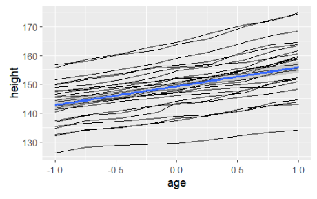
- 파란선이 잘보이기 위해 size 지정, se=false로 신뢰구간 표시x
- age와 height 간의 관계를 나타내며 subject에 따라 다른 의 선 그려짐
ggplot(Oxboys,aes(age,height))+geom_line(aes(group=Subject))+geom_smooth(method='lm',se=FALSE,size=2)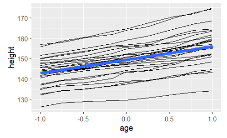
- 각 occasion별 boxplot
ggplot(Oxboys,aes(Occasion,height))+geom_boxplot()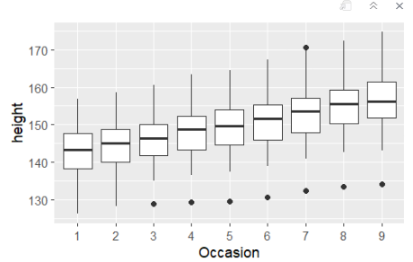
ggplot(Oxboys,aes(Occasion,height))+geom_boxplot()+geom_line(colour='#3366FF',alpha=0.5)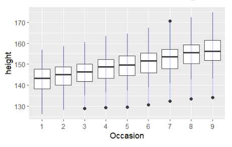
ggplot(Oxboys,aes(Occasion,height))+geom_boxplot()+geom_line(aes(group=Subject))
- color와 투명도(alpha) 추가
ggplot(Oxboys,aes(Occasion,height))+geom_boxplot()+geom_line(aes(group=Subject),color='blue',alpha=0.5)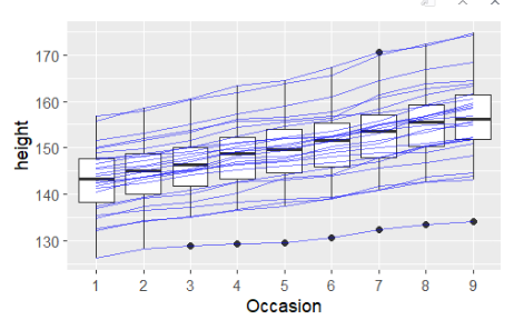
ggplot(Oxboys,aes(age,height))+geom_boxplot(aes(group=Occasion))- color 사용 예제
df = data.frame(x=1:3, y=1:3, colour=c(1,3,5))

df
ggplot(df,aes(x,y,color=factor(colour)))+geom_line()+geom_point()
ggplot(df,aes(x,y,colour=factor(colour)))+geom_line(aes(group=1),size=2)+geom_point(size=5)
- colour은 그룹과 차트를 묶어줌
ggplot(df,aes(x,y,colour=factor(colour)))+geom_line(aes(group=1),linewidth=2)+geom_point(size=5)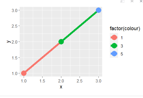
ggplot(mpg,aes(class))+geom_bar()
- fill = drv를 사용하여 drv 변수에 따라 막대의 색상을 구분
ggplot(mpg,aes(class))+geom_bar(aes(fill=drv))
- position = 'dodge'를 설정하여 막대를 겹치지 않고 나란히 표시
ggplot(mpg,aes(class))+geom_bar(aes(fill=drv),position='dodge')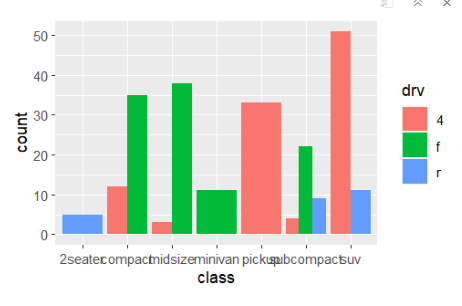
- theme을 활용하여 x축의 label을 조정
ggplot(mpg,aes(class,fill=drv))+geom_bar()+theme(axis.text.x=element_text(angle=45,hjust=1))- theme(axis.text.x = element_text(angle = 45, hjust = 1))
- 그래프의 x 축 레이블 텍스트를 45도 기울여 표시
- hjust = 1을 사용하여 레이블을 오른쪽 정렬
→ 이렇게 하면 x 축 레이블이 긴 경우에도 잘 보이도록 조정됨

geom_title() : data point가 중앙에 오는 title을 그려줌
geom_raster(stat='identity') : tile의 크기가 모두 같게 조정
geom_rect() : xmin, xmax, ymin, ymax로 지정되는 tile 그려줌
df <- data.frame(x = c(1, 2, 3), y = c(4, 5, 6), label = c("A", "B", "C"))p <- ggplot(df, aes(x, y, label = label)) + labs(x = NULL, y = NULL)p+geom_tile()+geom_point(color='yellow',size=4)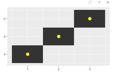
p+geom_raster()+geom_point(color='yellow',size=4)
p+geom_rect(aes(xmin=2.5,xmax=10,ymin=4,ymax=8))+ggtitle('rect')
head(faithful)
?faithfulOld Faithful Geyser Data
Description
Waiting time between eruptions and the duration of the eruption for the Old Faithful geyser in Yellowstone National Park, Wyoming, USA.
Usage
faithfulFormat
A data frame with 272 observations on 2 variables.
| [,1] | eruptions | numeric | Eruption time in mins |
| [,2] | waiting | numeric | Waiting time to next eruption (in mins) |
Details
A closer look at faithful$eruptions reveals that these are heavily rounded times originally in seconds, where multiples of 5 are more frequent than expected under non-human measurement. For a better version of the eruption times, see the example below.
There are many versions of this dataset around: Azzalini and Bowman (1990) use a more complete version.
dim(faithful)[1] 272 2→ 272번을 측정한 자료
faithfuld
ggplot(faithfuld,aes(eruptions,waiting))+geom_contour(aes(z=density,colour=after_stat(level)))
- geom_raster: x와 y를 내가 갖고 있는 값으로 처리함, 히트맵을 생성하는 지오메트리를 나타냄
ggplot(faithfuld,aes(eruptions,waiting))+geom_raster(aes(fill=density))
- faithfuld는 데이터셋을 나타냄
- aes(eruptions, waiting)은 x축에 eruptions 변수를, y축에 waiting 변수를 매핑
- geom_raster는 히트맵을 생성하는 지오메트리를 나타냄
- aes(fill = density)는 density 변수를 히트맵의 색상으로 매핑
→ 따라서 이 코드를 실행하면 faithfuld 데이터셋에서 eruptions와 waiting 변수의 관계를 시각화한 히트맵 그래프가 생성됩니다. density 값에 따라 색상이 다르게 표시됨/ 0.03쪽에 자료가 많은 것을 확인 가능
dim(faithfuld)- seq로 데이터를 일부만 추출 후 small 변수에 저장
seq(1,nrow(faithfuld),by=10)
small = faithfuld[seq(1,nrow(faithfuld),by=10),]
- seq(1, nrow(faithfuld), by = 10)를 사용하여 데이터셋에서 매 10번째 행을 선택하여 small 데이터셋을 만든다
small = faithfuld[seq(1,nrow(faithfuld),by=10),]
ggplot(small,aes(eruptions,waiting))+geom_point(aes(size=density))
- geom_point(aes(size = density))는 산점도를 생성하는 지오메트리를 나타내며, density 변수를 포인트의 크기로 매핑
→ 따라서 이 코드를 실행하면 faithfuld 데이터셋에서 선택한 행의 eruptions와 waiting 변수를 이용한 산점도가 생성됩니다. density 값에 따라 포인트의 크기가 다르게 표시됨
ggplot(small, aes(eruptions, waiting)) +
  geom_point(aes(size = density, alpha = 1/3)) +
  scale_size_area()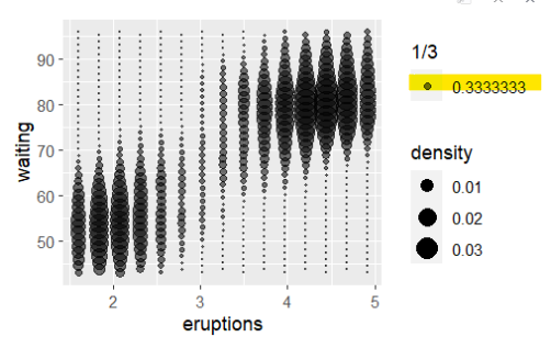
Text Mining이란?
- 자연어로 구성된 비정형 데이터에서 패턴 또는 관계를 추출하여 의미있는 정보를 찾아내는 기법
- 컴퓨터가 사람들이 말하는 언어를 이해할 수 있는 자연어 처리(natural language processing)에 기반을 둔 기술
- 텍스트에 나타나는 단어를 분해, 저제하고, 특정 단어의 출현빈도 등을 파악하여 단어들 간의
관계를 조사하는 기법
Word Cloud이란?
- 텍스트에서 빈번히 사용된 키워드를 시각적으로 표시하는 텍스트마이닝 방법
- 단어의 사용빈도가 높을수록 그 단어를 강조하기 위해 크게 표시하여 문서에서 강조하고자 하는
말을 한눈에 알아볼 수 있도록 하는 비주얼기법
library(tm)
library(wordcloud)

textMining = readLines("./data/wikipedia.txt")
myCorpus<- VCorpus(VectorSource(textMining))
myCorpus <- tm_map(myCorpus, stripWhitespace)
myCorpus <- tm_map(myCorpus, tolower)
myCorpus <- tm_map(myCorpus, removePunctuation)
myCorpus <- tm_map(myCorpus, removeNumbers)
myCorpus <- tm_map(myCorpus, removeWords, stopwords("english"))- space 없애기, 모두 소문자로 바꾸기, 컴마 점 없애기, 숫자자료 없애기
myCorpus <- tm_map(myCorpus, PlainTextDocument)
tdm<- TermDocumentMatrix(myCorpus)
m <- as.matrix(tdm)
myCorpus <- tm_map(myCorpus, PlainTextDocument)
tdm<- TermDocumentMatrix(myCorpus)
m <- as.matrix(tdm)
pal=brewer.pal(8,"Dark2")
set.seed(1234) # to make it reproducible
wordcloud(words=names(wordFreq), freq=wordFreq, scale=c(10,.5), min.freq=2,colors=pal, ra
ndom.order=F)
- shakespeare 문장에서 텍스트 마이닝 작업 해보기
shakespeare = readLines("./data/shakespeare.txt")
#length(shakespeare)
#head(shakespeare)
#tail(shakespeare)

shakespeare = shakespeare[-(124369:length(shakespeare))]
shakespeare = shakespeare[-(1:174)]
#length(shakespeare)

shakespeare = paste(shakespeare, collapse = " ")
#length(shakespeare)

shakespeare = strsplit(shakespeare, "<<[^>]*>>")[[1]]

(dramatis.personae <- grep("Dramatis Personae", shakespeare, ignore.case = TRUE))

## [1] 2 8 11 17 23 28 33 43 49 55 62 68 74 81 87 93 99 105 111
## [20] 117 122 126 134 140 146 152 158 164 170 176 182 188 194 200 206 212

#length(dramatis.personae)
shakespeare = shakespeare[-dramatis.personae]

myCorpus <- VCorpus(VectorSource(shakespeare))
myCorpus <- tm_map(myCorpus, tolower)
myCorpus <- tm_map(myCorpus, removePunctuation)
myCorpus <- tm_map(myCorpus, removeNumbers)
#myCorpus <- tm_map(myCorpus, removeWords, stopwords("english"))
myStopwords <- c(stopwords('english'), "thou", "let","shall",
"thee", "thy", "will", "now", "sir", "now", "well", "upon", "one", "tis", "may", "yet",
"must", "enter")

# remove stopwords from corpus
myCorpus <- tm_map(myCorpus, removeWords, myStopwords)
myCorpus <- tm_map(myCorpus, PlainTextDocument)

tdm <- TermDocumentMatrix(myCorpus)
m <- as.matrix(tdm)

wordFreq <- sort(rowSums(m), decreasing=TRUE)

pal=brewer.pal(8,"Dark2")

set.seed(1234) # to make it reproducible
wordcloud(words=names(wordFreq), freq=wordFreq, min.freq=500, colors=pal, random.order=F)
감성분석이란?
- 텍스트를 작성한 사람들의 태도, 의견, 성향과 같은 주관적인 데이터를 가지고 특정 주제에 대해
긍정인지 또느느 부정인지를 분류하는 기술 - opinion mining 이라고도 함.
- 감성점수 = 긍정적 리스트, 부정적 리스트 만들기 → (단어의 수 - 부정적 단어의 수) 계산하기
– 긍정적 단어, 부정적 단어에 대한 정의가 필ㅇ
– 감성점수 >0 : 대체로 긍정적인 의견을 나타내는 문서로 간주
– 감성점수 <0 : 대체로 부정적인 의견을 나타내는 문서로 간주
– 감성점수 =0 : 대체로 중립적인 의견을 나타내는 문서로 간주
library(twitteR)
library(plyr)

##
## Attaching package: 'plyr'

## The following object is masked from 'package:twitteR':
##
## id

library(stringr)

score.sentiment = function(sentences, pos.words, neg.words)
{

 # Parameters
 # sentences: vector of text to score
 # pos.words: vector of words of postive sentiment
 # neg.words: vector of words of negative sentiment
 # create simple array of scores with laply

 scores = laply(sentences,
 function(sentence, pos.words, neg.words)
 {

 # remove punctuation
 sentence = gsub("[[:punct:]]", "", sentence)
 # remove control characters
 sentence = gsub("[[:cntrl:]]", "", sentence)
 # remove digits?
 sentence = gsub('\\d+', '', sentence)

 # define error handling function when trying tolower
 tryTolower = function(x)
 {

 # create missing value
 y = NA
 # tryCatch error
 try_error = tryCatch(tolower(x), error=function(e) e)
 # if not an error
 if (!inherits(try_error, "error"))
 y = tolower(x)
 # result
 return(y)
 }

 # use tryTolower with sapply
 sentence = sapply(sentence, tryTolower)

 # split sentence into words with str_split (stringr package)
 word.list = str_split(sentence, "\\s+")
 words = unlist(word.list)

 # compare words to the dictionaries of positive & negative terms
 pos.matches = match(words, pos.words)
 neg.matches = match(words, neg.words)

 # get the position of the matched term or NA
 # we just want a TRUE/FALSE
 pos.matches = !is.na(pos.matches)
 neg.matches = !is.na(neg.matches)

 # final score
 score = sum(pos.matches) - sum(neg.matches)
 return(score)
 }, pos.words, neg.words)

 # data frame with scores for each sentence
 scores.df = data.frame(text=sentences, score=scores)
 return(scores.df)
}

pos.words = scan('./data/positive-words.txt', what='character', comment.char=';')
neg.words = scan('./data/negative-words.txt', what='character', comment.char=';')
#pos.words = c(hu.liu.pos)
#neg.words = c(hu.liu.neg)

sample = c("You're awesome and I love you",
"I hate and hate and hate. So angry. Die!",
"Impressed and amazed: you are peerless in your achievement of unparalleled mediocrity",
"Oh how I love being ignored",
"Absolutely adore it when my bus is late.")

result = score.sentiment(sample, pos.words, neg.words)

library(ggplot2)

##
## Attaching package: 'ggplot2'

## The following object is masked from 'package:NLP':
##
## annotate

plot.data<-data.frame(score=result$score)
ggplot(plot.data,aes(score))+geom_histogram()
## `stat_bin()` using `bins = 30`. Pick better value with `binwidth`
'Data visualization > 데이터시각화(R)' 카테고리의 다른 글
| 데이터시각화(R)_USA-covid19 (0) | 2023.10.03 |
|---|---|
| 데이터시각화(R)_Covid19 (0) | 2023.10.02 |
| 데이터시각화(R)_Diamonds (1) | 2023.09.20 |
| 데이터시각화(R)_Penguins (1) | 2023.09.16 |
| 데이터시각화(R)_Iris Code (0) | 2023.09.15 |