Diamonds: 53,940 개의 다이아몬드에 대한 자료
- 변수들
- carat: 다이아몬드 무게(lb)
- cut: 절단면에 대한 품질 (Fair, Good, VeryGood, Premium, Ideal)
- color: 다이아몬드 색깔 (D:best ~ J:worst) - clarity: 다이아몬드의 맑고 깨끗한 정도 (I1:worst, SI2, SI1, VS2, VS1, VVS2, VVS1, I F:best)
- depth: 깊이 = 2*z/(x+y)
- table: 상단면
- price: 다이아몬드 가격(dollar)
- x: length
- y: width
- z: depth
library(tidyverse)
diamonds
ggplot(diamonds,aes(depth))+geom_histogram()
range(diamonds$depth)[1] 43 79ggplot(diamonds, aes(depth)) +
geom_histogram()+
xlab(quote(paste("depth=2*",frac(z,(x+y)))))
ggplot(diamonds, aes(depth)) +
 geom_histogram(binwidth = 0.1) +
 xlim(55, 70)
- depth를 cut별로 비교해보기
ggplot(diamonds, aes(depth)) +
 geom_freqpoly(aes(colour = cut), binwidth = 0.1
- 58부터 68까지만 비교해보기
ggplot(diamonds, aes(depth)) +
 geom_freqpoly(aes(colour = cut), binwidth = 0.1, na.rm = TRUE) +
 xlim(58, 68)
- na.rm : not available을 다 삭제
- theme으로 legend.position 모두 삭제
ggplot(diamonds, aes(depth)) +
 geom_freqpoly(aes(colour = cut), binwidth = 0.1, na.rm = TRUE) +
 xlim(58, 68) +
 theme(legend.position = "none")
- fill=cut별로 나누면 보기가 어렵기 때문에, position='fill'사용
ggplot(diamonds,aes(depth))+geom_histogram(aes(fill=cut))
ggplot(diamonds,aes(depth))+geom_histogram(aes(fill=cut),position='fill')
- geom_histogram(position = "fill") 이용하여 범주별로 분포 비교하기
ggplot(diamonds, aes(depth)) +
 geom_histogram(aes(fill = cut),
 binwidth = 0.1,
 position = "fill",
 na.rm = TRUE) +
 xlim(58, 68) +
 theme(legend.position = "none")
- geom_density()를 이용하여 범주별로 분포 비교
ggplot(diamonds,aes(depth,fill=cut))+geom_density()
ggplot(diamonds, aes(depth, fill = cut, colour = cut)) +
 geom_density(alpha = 0.2, na.rm = TRUE) +
 xlim(58, 68)
- geom_boxplot()을 이용한 평행 상자 그림
ggplot(diamonds, aes(clarity, depth)) +
 geom_boxplot()
- cut_width()를 이용하여 연속변수를 범주화
ggplot(diamonds, aes(carat, depth)) +
 geom_boxplot(aes(group = cut_width(carat, 0.1))) +
 xlim(NA, 2.05)
- geom_violin()을 이용하여 범주별로 분포 비교하기
ggplot(diamonds, aes(clarity, depth)) +
 geom_violin()
- 자료의 수가 많아지는 문제점: 점들이 겹쳐보임
1) 예시 만들기
df <- data.frame(x = rnorm(2000), y = rnorm(2000))
head(df)
x y
1 -1.1035419 0.1390348
2 -0.7344715 -0.9664105
3 -0.8875536 -0.9620061
4 -1.8759312 -0.9459027
5 1.0572611 0.9014619
6 0.3740912 1.0429716첫 번째 방법: 점 분산으로 겹쳐보이는 것 해결
norm <- ggplot(df, aes(x, y)) + xlab(NULL) + ylab(NULL)
norm + geom_point()
norm + geom_point(shape = 1)
norm + geom_point(shape = ".")
두 번째 방법: alpha를 이용하여 투명도 조절
norm + geom_point(alpha = 1 / 10)
2 차원 binning 을 이용하여 점이 겹쳐지는 정도를 농도로 나타내기
norm + geom_bin2d()
norm + geom_bin2d(bins = 10)
- 낮은 쪽은 무슨 색으로 할지, 높은 쪽은 무슨 색으로 할지 지정
norm + geom_bin2d()+scale_fill_gradient(low="black",high="white")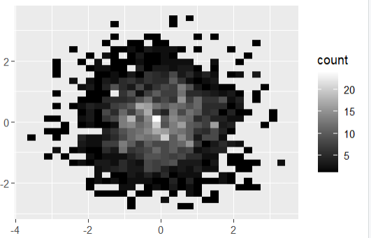
Statistical summaries
ggplot(diamonds, aes(color)) + geom_bar()
ggplot(diamonds, aes(color, price)) +
 geom_bar(stat = "summary_bin",fun="mean")
→ d칼라가 제일 good!
geom_bin2d : 2차원 히스토그램
ggplot(diamonds, aes(table, depth)) +
  geom_bin2d()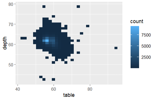
ggplot(diamonds, aes(table, depth)) +
 geom_bin2d(binwidth = 1, na.rm = TRUE) +
 xlim(50, 70) + ylim(50, 70)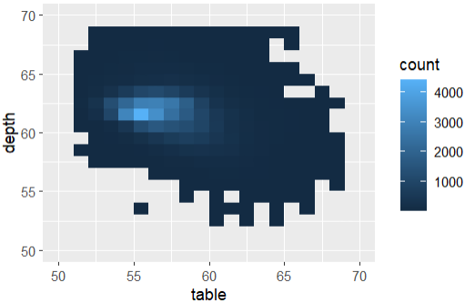
- stat="summary_2d" 이용하여 table, depth 별로 price 평균을 나타내기
ggplot(diamonds, aes(table, depth,
 z = price)) +
 geom_tile(binwidth = 1,
 stat = "summary_2d",
 fun = mean, na.rm = TRUE) +
 xlim(50, 70) + ylim(50, 70)
- 산점도 위에 통계량을 함께 표시
ggplot(mpg, aes(trans, cty)) +
 geom_point() +
 stat_summary(geom = "point", fun = "mean", colour = "red", size = 4)
- geom='point' : 통계 요약을 점으로 나타냄
- fun='mean' : 각 그룹의 평균 계산
- size = 4 : 점 크기 지정

- `..count..`: 각 범주의 관측수
- `after_stat(density)`:각 범주의 관측에 대한 비율 (percentage of total / bar width)
- `..x..`: 각 범주의 중심
ggplot(diamonds, aes(price)) +
 geom_histogram(binwidth = 500)
ggplot(diamonds, aes(price)) +
 geom_histogram(aes(y = after_stat(density)), binwidth = 500)
ggplot(diamonds, aes(price, colour = cut)) +
 geom_freqpoly(binwidth = 500) +
 theme(legend.position = "none")
여러가지 지정사항들 바꾸기
- label: xlab() 과 ylab()을 이용
ggplot(mpg, aes(cty, hwy)) +
 geom_point()
ggplot(mpg, aes(cty, hwy)) +
 geom_point() +
 xlab("city driving (mpg)") +
 ylab("highway driving (mpg)")
- Remove the axis labels with NULL
ggplot(mpg, aes(cty, hwy)) +
 geom_point() +
 xlab(NULL) +
 ylab(NULL)
df <- data.frame(x = c(1, 3, 5) * 1000, y = 1)
axs <- ggplot(df, aes(x, y)) +
 geom_point() +
 labs(x = NULL, y = NULL)
axs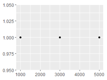
axs + scale_x_continuous(breaks = c(2000, 4000))
'Data visualization > 데이터시각화(R)' 카테고리의 다른 글
| 데이터시각화(R)_Tips (1) | 2023.10.15 |
|---|---|
| 데이터시각화(R)_Diamonds (1) | 2023.10.14 |
| 데이터시각화(R)_Shiny (0) | 2023.10.03 |
| 데이터시각화(R)_USA-covid19 (0) | 2023.10.03 |
| 데이터시각화(R)_Covid19 (0) | 2023.10.02 |